An Overview of Rollup
Rollup is a category of blockchain Layer 2 scaling solutions. In Rollup schemes, operators of the project run a relatively independent Layer 2 platform underneath the expanded main chain (i.e., Layer 1). Users can execute contracts or transfer tokens on the Layer 2 platform.
The security of the Layer 2 platform is guaranteed by the Layer 1 blockchain it relies on. When a new block is generated in Layer 2, the transaction information from the Layer 2 block, as well as the post-transaction state root of Layer 2, are bundled as a Rollup transaction and published on the Layer 1 chain. The actual transaction execution and state changes are processed on the Layer 2 platform below the main chain, and Layer 1 only needs to verify the correctness of the state transitions of Layer 2. Since the cost of verifying state transition correctness is much lower than executing these transactions on Layer 1, Layer 2 can achieve an expansion of the Layer 1 platform. The Layer 2 platform can offer higher transaction throughput and lower transaction costs compared to Layer 1 while maintaining equivalent security.
Compared to other off-chain transaction schemes, Rollups have two characteristics:
- The availability of state data for the second layer is solved by storing it on the main chain. The Layer 2 platform records all transaction information or complete Layer 2 state changes in blocks on the main chain. Should the Layer 2 state be lost, anyone can recover the missing state from the information stored on the main chain.
- In the Rollup scheme, the Layer 2 state root changes packaged and stored on the main chain need to be verified in some way on the main chain. After verification, the state of Layer 2 will be locked on the Layer 1 main chain. Therefore, under the condition of a secure verification scheme, Layer 2 can enjoy the same level of security as Layer 1.
Based on the verification methods of Layer 2 state updates by the main chain, there are currently two main types of Rollup technology solutions. One is Optimistic Rollup. In this type of scheme, the main chain contract does not directly verify the new state submitted by Layer 2. Instead, a challenge period is prepared for each new state submitted. Since Rollup submits all transaction information to the main chain and makes it public, anyone can verify the state update (especially when the update involves their own wallet). If the new state is incorrect, a verifier can generate a fraud proof against that erroneous state and submit it within the challenge period, thus invalidating the incorrect state update.
Another type of Rollup solution is zk Rollup. In this type of scheme, after executing the Layer 2 state update, the operator of Layer 2 must provide a zero-knowledge proof of the correctness of the state update and submit it to the main chain along with the state update. The contract on the main chain will verify the proof to determine the correctness of the state update.
Compared to the Optimistic Rollup scheme, zk Rollup does not require a lengthy challenge period to finally confirm Layer 2 transactions and can be confirmed more quickly. In addition, zk Rollup does not rely on the assumption that there will always be honest verifiers in the network who will timely submit fraud proofs when fraud occurs. However, at the same time, zk Rollup also faces issues such as the high computational cost of zero-knowledge proof technology, complexity, and difficulty in development, which hinder the practical implementation of zk Rollup technology in Rollups. With the further development of zero-knowledge proof technology in the past two years, these obstacles are gradually being overcome. zk Rollup technology is starting to occupy an increasingly large share of the Layer 2 market.
As shown in the figure below, within the Rollup layer-2 scaling field, zkRollup already occupies more than half of the territory and is rapidly developing.
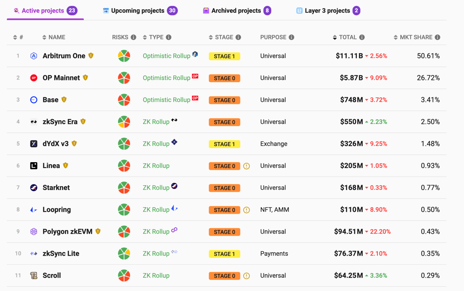
Image source
Data retrieved on: January 18, 2024
From Specialized zkRollup to General zkRollup
During its development, zkRollup has mainly gone through two stages. The first type is the non-general zkRollup, while the second type is the general zkRollup capable of executing Turing-complete arbitrary contracts.
The difference between these two types of zkRollup technology mainly lies in whether the Layer 2 platform executes limited specialized logic written by the platform provider or arbitrary smart contract logic written by users in transactions.
In non-general zkRollup projects (like zkSync Lite, which ranks 8th in the figure above), users can only perform a few types of transaction operations, such as FT (fungible token) transfers, payments, swaps, and NFT (non-fungible token) transfers. The transaction logic for these operations can only be defined and implemented by the project owners.
Through such zkRollup projects, we can transfer with much lower fees compared to the Ethereum mainnet and obtain higher transaction throughput. However, if we want to try out some interesting contract on the chain, we will not be able to do so.
Why can’t specialized zkRollups allow users to deploy and use their own smart contracts? This brings us back to the proof architecture of zkRollup itself.
To ensure that the state transitions of L2 are correct and trustworthy, in zkRollup, all L2 state transition logic needs to be written as zero-knowledge proof circuits and verified by the L1 contracts. Only states that pass verification can be accepted by L1 and ultimately complete the Rollup. This process requires that all transaction execution logic of the zkRollup platform is verified in the zero-knowledge proof circuit. However, supporting the execution of arbitrary contract logic in zero-knowledge proof circuits is a challenge (the reasons for this difficulty will be explained later in the text). As a result, early zkRollup projects often only supported a limited number of relatively simple transactions.
Being able to execute only a fixed number of simple transactions obviously does not meet our expectations for zkRollup. Fortunately, zkVM (Zero-Knowledge Virtual Machine) technology has solved the difficulty of proving the execution of any arbitrary Turing-complete code within zero-knowledge proof circuits, making the general zkRollup platform a possibility. Next, this article will introduce the implementation principles of zkVM, allowing readers to understand how this most core part of general zkRollup technology operates.
The Implementation Principles of zkVM
Before introducing the principles of zkVM, we will first provide a brief introduction to zero-knowledge proof technology. Here, we don’t need a detailed understanding of the underlying mathematical principles of zero-knowledge proofs; it’s enough to understand what zero-knowledge proofs can do, how they are used, and the limitations imposed by their specialized proof circuits.
An Introduction to Zero-Knowledge Proofs
Zero-knowledge proofs in zkRollup serve to prove that Layer 2 transactions have been executed correctly and that the state of Layer 2 has been updated correctly.
To achieve this purpose, the zkVM circuit needs to prove that any smart contract deployed on Layer 2 has been executed correctly. Before introducing the principles of zkVM, we need to first discuss the role of zero-knowledge proofs and how they work.
Why Zero-Knowledge Proofs Are Needed
Zero-knowledge proof is a cryptographic primitive that allows a prover to convince a verifier of the correctness of a statement without revealing any additional information to the verifier.
Zero-knowledge proofs have three core properties:
- Completeness: If the statement to be proven is true, an honest verifier (that is, one following the protocol properly) will be convinced of this fact by an honest prover.
- Soundness: If the statement to be proven is false, a dishonest prover has only a negligible chance of convincing the honest verifier that it is true.
- Zero-knowledge: Besides the statement being true, the verifier cannot obtain any additional information from the verification process.
With the completeness of zero-knowledge proofs, when the prover completes a complex calculation, they can produce a proof that convinces the verifier that the output data obtained from the input data is the result provided by the executor. The soundness of zero-knowledge proofs ensures that when the executor provides a wrong result, they cannot generate a valid proof.
Therefore, with the completeness and soundness of zero-knowledge proofs, we can confidently outsource these complex calculations to others and verify through a relatively simple verification process whether the calculation is correct, without needing to trust the outsourced party.
In addition to the three core properties of zero-knowledge proofs, the widely used zk-SNARK scheme also have the characteristic of succinctness. This means that for any complex logic that is proven using zero-knowledge proofs, the size of the proof generated and the time taken to verify the proof are both fixed and relatively small. This allows the zk-Rollup to offload state update calculations off-chain and only verify the correctness of operations on-chain, making the scaling solution feasible.
The Process of Zero-Knowledge Proofs
Next, this article will use the simple calculation below as an example to explain the process of zero-knowledge proofs.
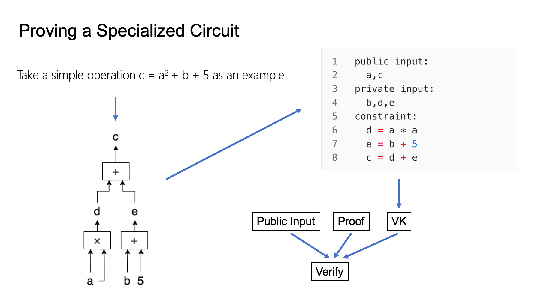
$c=a^2+b+5$
For the sake of explaining the zero-knowledge aspect in zero-knowledge proofs, we will set variables a and c as the public values of this zero-knowledge proof, with b as the secret input known only to the prover. Since our calculation is very simple, the verifier can easily deduce the value of the secret input from the public values. This does not affect the zero-knowledge property of the zero-knowledge proof method itself, as it only guarantees that the verifier cannot obtain information about the secret input from the proof process.
When proving, the prover first selects a value for a and b respectively as inputs and calculates the value of c. Here, we set a = 3, b = 2, then c = 16. After completing all calculations, the prover can generate a zero-knowledge proof for these values and operations.
After completing the proof, the prover will give the verifier the public inputs of the proof (i.e., the values of a and c) as well as the zero-knowledge proof.
Upon receiving the proof, the verifier can, by validating the zero-knowledge proof, be convinced that the prover has used a secret input b, which makes the above formula true when a = 3 and c = 16 (i.e., the public input values), and is unable to obtain any information beyond the public inputs (a = 3, c = 16).
The next part of the article will introduce the specific proof process. When we need to prove a computation using the zero-knowledge proof method, we first need to represent the computation in the form of an arithmetic circuit that the zero-knowledge proof algorithm can accept. Arithmetic circuits are Turing-complete representations of computation. As the name implies, an arithmetic circuit is a computational circuit made up of gates that perform arithmetic operations. In our example, the conversion result is shown in the figure. You may notice that in addition to the public inputs a and c and secret input b we mentioned, there are two additional values, d and e. These are intermediate variables used in the computation process.
We can think of each wire in the arithmetic circuit as a value, which could be a public input, a secret input, or an intermediate variable. After expanding the computation into an arithmetic circuit, each intermediate variable will have its place and be used in the proof process. The only difference between them and the inputs is that their values are not directly entered by the prover but determined by other input values in the arithmetic circuit.
We can see the arithmetic circuit as two parts: one part is all the numerical values that appear in the circuit, and the other part is the relationships (constraints) between these values. We usually refer to the public inputs in the circuit as the statement (in our example, a and c), and all other values, including the secret inputs (b) and intermediate variables (d and e), as the witness.
According to the logic of the circuit, when we have the public inputs as the statement and the secret inputs as the witness, we can calculate all the witness values in the circuit.
Therefore, the gate circuit of the arithmetic circuit can also be represented in the following form:
1 | statement: |
After the circuit to be proven is arithmetized, the zero-knowledge proof algorithm needs to process the circuit’s constraints and convert them into the form required by the algorithm for the generation and validation of proofs. After processing, the circuit produces a fixed-length VK (Verification Key) that is unrelated to the size of the circuit. The verifier can verify the zero-knowledge proof of the corresponding circuit through the verification key. The verification key is somewhat similar to a commitment to the circuit. If any changes occur to the constraints, the corresponding verification key will also change.
In actual applications, users of zero-knowledge proofs need to write the logic they require into zk circuit source code and generate a corresponding VK through auditing. This VK is handed over to the verifier. The public inputs proven by the prover, along with the generated proof, are submitted, and the verifier can verify whether these public inputs meet the constraints. In this example, the prover can generate a proof with the values of a, b, and c. The verifier can verify whether a2 + b equals C without performing this operation.
Limitations of Zero-Knowledge Proof Circuits
Although zk circuits are Turing-complete and can represent any computation, due to the need to convert computations into the special representation form of arithmetic circuits, there are some additional restrictions in writing arithmetic circuits.
In computer programs we are more familiar with, we can control the branches of program execution with if-else statements. Only the selected branch in the program is executed. However, in the zero-knowledge proof process, computations are flattened into circuits, and there is no concept of execution paths or control flows. Thus, we cannot choose a particular branch to execute in an arithmetic circuit.
Of course, this does not mean that we cannot use branches and selections in circuits. It just means that in circuits, all branches, whether selected or not, will be executed and contribute to the production of the proof. The selection of branches only affects which branch’s result will be output to the next variable.
Take the following operation as an example:
1 | if (flag) { |
When this operation is converted into an arithmetic circuit, it will be converted into the constraints shown below. Obviously, two new witnesses, temp1 and temp2, will be added to the circuit. In addition, the value of x+x and the value of x*x will both be calculated.
That is, in a zk circuit, all branches and logic will be computed, whether they are executed or not.
1 | temp1 = x + x |
Because of these limitations, supporting conditional selection in zero-knowledge proof circuits is quite difficult. How to prove the execution path of a smart contract logic with many variations in a zero-knowledge proof is one of the main challenges of a zk virtual machine.
Proving the Execution of Any Program - Proving a Universal State Machine in a Circuit
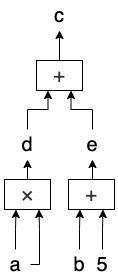
We describe the VM through a model of a universal state machine. A VM is a state machine that transitions states as instructions are processed. Let’s illustrate how a virtual machine is proven by a zero-knowledge circuit with a very simple state machine example.
We assume this universal state machine has general-purpose registers (A and B), and additionally, a Program Counter register that stores the current instruction number.
The state of the registers before executing instruction $i$ is $A^i, B^i$, which, after the execution of instruction $i$, transitions to state $A^{i+1}, B^{i+1}$.
The figure below shows the basic workflow of a ZK virtual machine proving circuit:
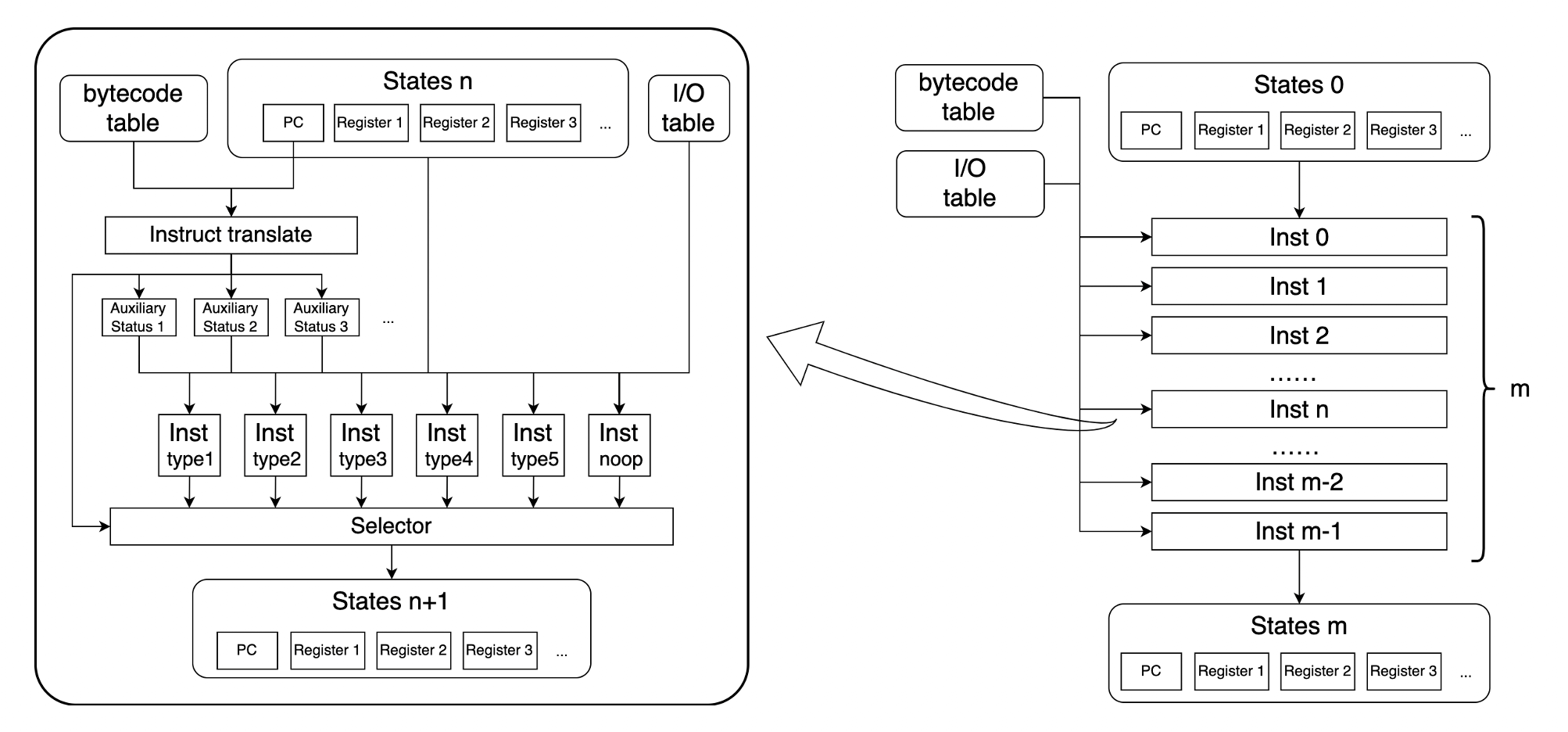
State 0 can be considered the initial state of this virtual machine before running. The initial state, after a total of m instructions, reaches the final state m. In addition to the initial state, this virtual machine has two regular input tables:
- Bytecode Table: Stores the program executed in the state machine.
- I/O Table: Stores all inputs and outputs generated during the execution of the virtual machine.
In the figure, the execution process of the nth instruction is abstracted and displayed on the left. The state of the state machine, State n, transitions to State n+1 after the execution of the nth instruction. The same circuit, after m iterations, achieves the execution of m instructions in the vm.
There are two issues here.
One is how to execute different instructions within a fixed circuit? When executing contract bytecode, it’s not possible to determine what the nth instruction that is executed is, so the actual circuit logic here cannot be determined.
The second is how to prove if the number of instructions to be executed is not m?
For the first question, the solution is to implement the logic for all possible instructions in the circuit. Then use a Selector, based on the instruction, to choose one of them as the next state, similar to the if-else in the specialized circuit mentioned before.
For the second question, we cannot directly change the number of instructions in the circuit. This is because each instruction in the circuit requires an independent circuit segment to implement. If the number of instructions increases or decreases, the circuit will change, and the corresponding verification key will also change. This makes it impossible to meet the requirements for verifying any logic in a fixed circuit.
To solve this problem, a noop instruction which won’t change the state can be added to the instruction set. Therefore, there is an upper limit to the number of instructions that each fixed circuit can execute. The zkVM’s circuit can be seen as a container with a fixed number of instruction slots. If more instructions are needed, a larger circuit is required. In actual proof, a circuit of appropriate size can be selected as needed.
Proving a Basic Instruction
Here are some basic computational instructions as an example of how the basic instructions in the circuit are proven:
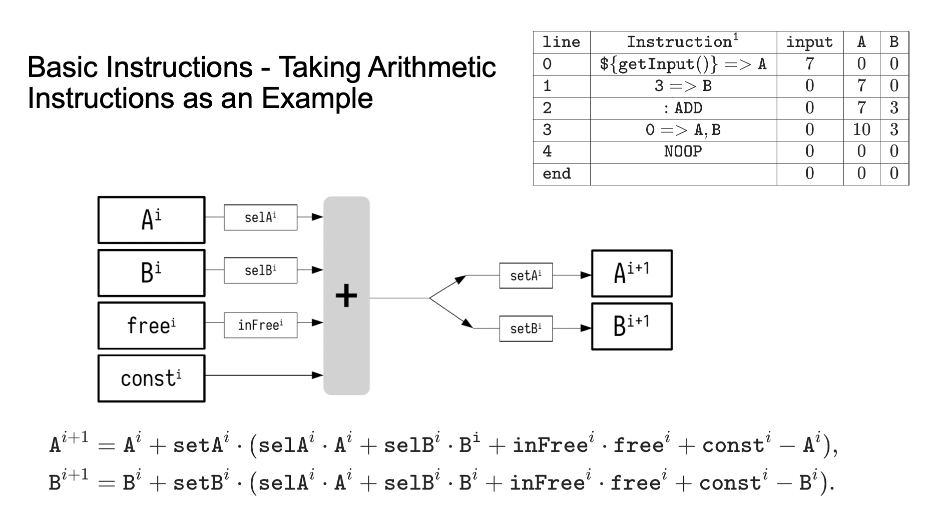
The figure shows the flowchart of the instruction proving circuit. The formulas below are the circuit constraints for the proof.
These two constraints can prove several basic instructions for the general-purpose registers A and B listed in the top right corner. These proofs can load values from the input table or immediate values from the instructions into the registers or add the values in registers A and B and write them back to the registers.
From this figure, we can see that in order to build constraints for state changes, the circuit introduces some auxiliary control states:
$selA, selB$ indicate whether to select registers $A, B$ as input
$inFree$ indicates whether to choose free as input
$setA, setB$ indicate whether to write the calculation result to registers $A, B$
The selected inputs and $const$ immediate values will be summed and then input into the output register selected by set.
When data needs to be read from the free input and written to the A register, $inFree$ and $setA$ are selected, so the value in free will be written into the A register, thus implementing the instruction to read input into the A register.
When an addition operation is needed, during the execution of line 3, $selA,selB$ are selected, so the values of registers $A,B$ are summed and then written to the register $A$ selected by $selA$, thus implementing the instruction for addition.
The computational logic between these auxiliary registers and general-purpose registers is implemented by the formulas below. Interested readers can substitute the corresponding values into the constraint formulas to verify. It can be seen that with these two constraints, basic arithmetic addition instructions can be implemented. If more operations are needed, more instruction constraints will have to be added.
Returning to the basic process diagram, we can regard the computational circuit in this section as an instruction in the overall process. The Selector will choose whether the result it produces is the next state to be adopted by the state machine. The auxiliary states required by the circuit in this section are generated by the instruction pointed to by the PC register.
Instruction retrieval is implemented by a specialized lookup circuit, which can prove the retrieval of a segment of data from a fixed table through an index. Therefore, the zkVM circuit can prove the state transition executed by the virtual machine specified by PC.
Proving Conditional Judgments and Control Flow Jumps
The state machine’s ability to execute complex logic relies on conditional and jump instructions. In actual contracts, we often need to deal with logic that changes the execution path based on conditions, so such circuits are necessary.
It should be noted here that zkVM circuits are not modules that actually execute contract logic and calculate results. What zkVM circuits actually do is prove the calculation process of the contract logic. Therefore, when proving, it is necessary to fill the actual executed instruction sequence process in the circuit, verify through the circuit whether the conditions for this jump are met, and then prove that the executed instruction flow has made the correct jump.
First, we introduce the proof of condition judgment:
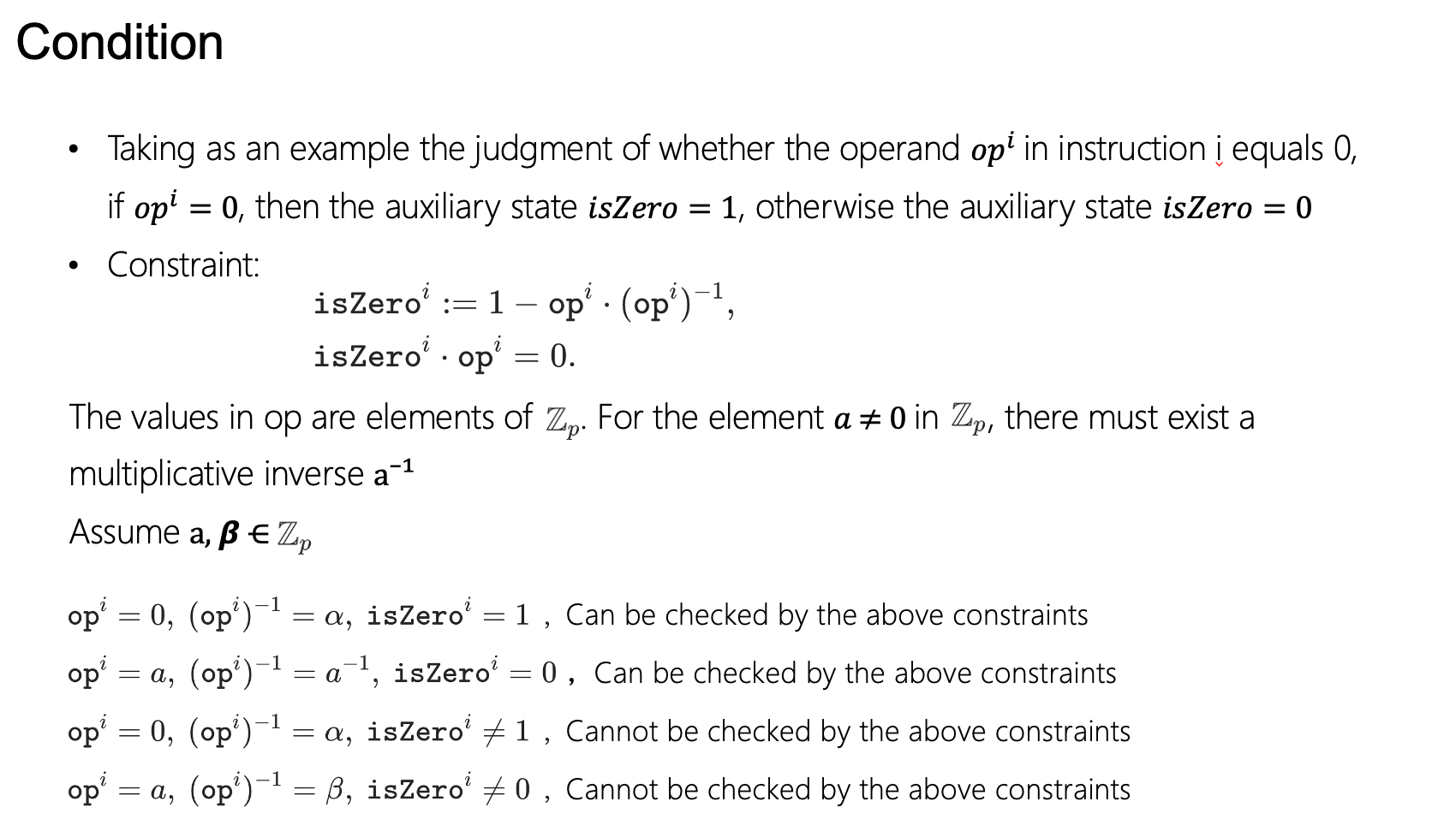
Taking the judgment of whether the operand in the ith instruction equals zero as an example. We add an auxiliary state isZero for the judgment result. If the judged value is 0, then the value of the auxiliary state isZero is 1; if the judged value is any other value besides 0, then isZero is 0.
This process is constrained by the two formulas in the diagram.
The validity of this constraint is related to the mathematical properties of the elliptic curves used in zero-knowledge proofs. Every value in a zero-knowledge proof circuit is an element within a finite field on an elliptic curve. If its value is not 0, there must be an inverse element that, when multiplied by itself, results in 1. Using this property, with the two constraints in the diagram, it is possible to verify whether a value is zero and convert it into an auxiliary state.
Once we have this isZero condition auxiliary state, we can proceed to the proof of conditional jump instructions:
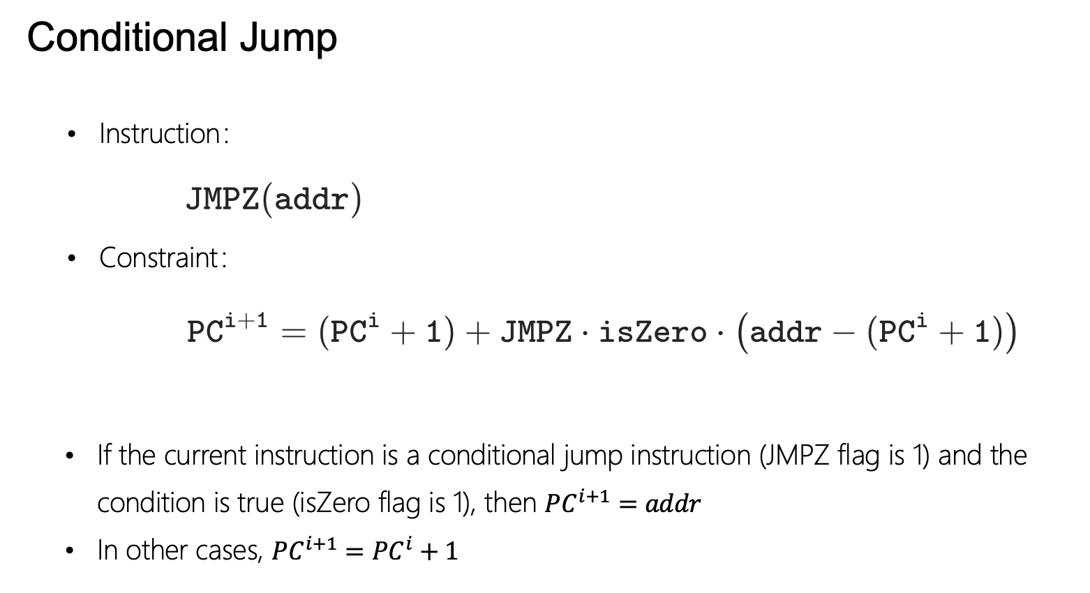
When executing the jump instruction $\mathtt{JMPZ(addr)}$, the circuit checks whether the value of $\mathtt{isZero}$ is 0; if it is, then the value of $\mathtt{PC}$ is changed to the value specified in the jump instruction. When the jump instruction is not executed, the value of $\mathtt{PC}$ is incremented by 1 each time, allowing the instructions to be executed sequentially. It can be seen that the jump instruction is actually an instruction that modifies the state of $PC$.
The implementation of this constraint can be achieved with the constraints in the diagram. It can be seen that only when $\mathtt{JMPZ, isZero}$ are both 1 will the value of $\mathtt{PC}$ be set to $\mathtt{addr}$; otherwise, it will only increment by one.
Returning to the basic process diagram, if the current instruction is a conditional jump instruction. It first carries out an isZero check, determines whether the jumping condition is met, and then modifies the value of PC. After updating the value of PC, the execution of the next instruction first involves a lookup based on PC to find the instruction after the jump.
I/O and Complex Operations
When using a general state machine proof circuit, to correctly handle state transitions, it is necessary to add corresponding control states and constraints for each supported instruction during a single state transition. The number of these state values and constraints must also be multiplied by the number of instructions supported by the zkVM. Even if no operations are performed in the actual program executed by the zkVM (all NOPs), these state values and constraint checks cannot be omitted.
Therefore, using the general state machine circuit in the first half of this article to execute complex calculations is very inefficient. If these methods are used to implement complex calculations, their performance is difficult to accept. In addition, it is difficult for the general state machine circuit to execute complex instructions or interact directly with the outside world.
To solve this problem, actual implementations of zkVMs typically use a combination of general state machine circuits and specialized proof circuits to prove parts of the program separately and then aggregate the proofs into one solution.
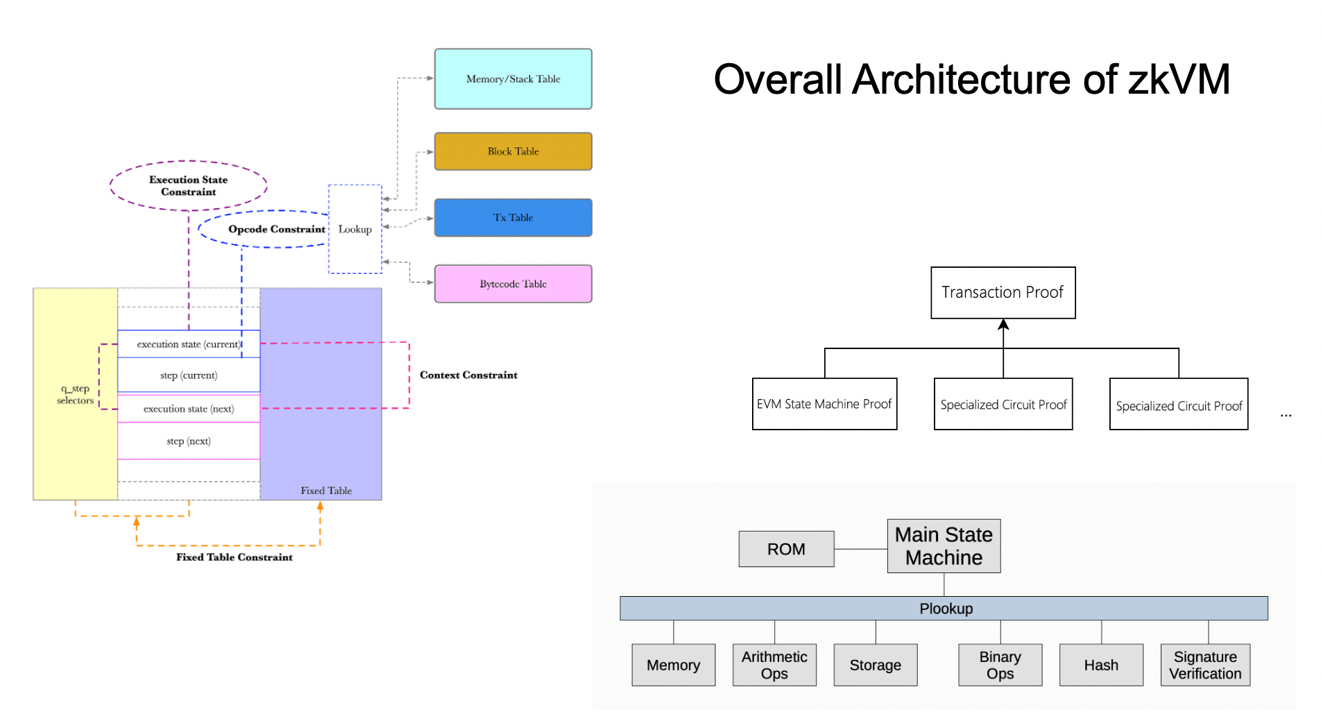
The diagram on the left is the circuit architecture of the Scroll project, and the diagram in the bottom right corner is the circuit architecture of Polygon. They both employ a similar approach as shown in the diagram in the top corner.
The general state machine is responsible for proving the execution logic control of the program. In most contracts, the actual execution time of this part of the logic is very small, so proving it with the inefficient general state machine is still acceptable in terms of efficiency.
More fixed complex calculations, such as hash, MPT tree operations, external input data, etc., are proven by specialized circuits.
The general state machine and specialized proof circuits interact using lookup tables. Every time the state machine circuit calls these operations, the modules that generate the witness for the proof will write the call parameters and calculation results in the lookup table. Thus the calls to these operations in the state machine circuit are simplified to a look up operation.
The correctness of each call and return value in the lookup table is constrained and proven by a specialized circuit.
Finally, the copying constraints in the circuit connect the state machine circuit, specialized circuits, and lookup tables, checking whether each item in the lookup table is proven by the corresponding specialized circuit, and ultimately generating a proof for the complete block.
The L1 contract only needs to verify this aggregate proof to confirm the correctness of the entire virtual machine execution process.
Conclusion
Zero-knowledge proof technology has made it possible to prove calculations simple and fastly, opening the door to outsourcing computational processes in a trustless environment. This technology, when used in blockchain, liberates execution from the chain, allowing the main blockchain to focus on decentralized and security issues. But the characteristic of specialized zero-knowledge proof circuits to execute only fixed logic limits the potential of zero-knowledge proofs on blockchain, confining the early zkRollup’s capabilities to a few types of transactions.
However, with the development and maturation of zk virtual machines, supporting Turing-complete execution of arbitrary smart contracts has become possible. The potential of zkRollup will be truly unleashed, realizing its vision of breaking the blockchain trilemma.
About
AntChain Open Labs
AntChain Open Labs is a research center initiated by AntChain and world leading computer scientists in the area of foundational trust technologies. It is dedicated to building a secure, transparent and reliable Web3 infrastructure driven by innovative research and aiming to advance transformative services.
Website:https://openlabs-intl.antdigital.com/home
ZAN
ZAN, powered by AntChain Open Labs, provides solutions for Web3, such as Smart Contract Review, KYT, KYC, Node Service, and more.
Website | Telegram | Discocd | Twitter | More